#loading packages

library(dplyr, warn.conflicts = FALSE)
library(ggplot2)
library(readr)
library(gridExtra, warn.conflicts = FALSE)CDC Data-Exercise
Loading and checking data
Data Description
The dataset, titled “NNDSS Table II. Tuberculosis - 2019”, is sourced from the Centers for Disease Control and Prevention (CDC) through their data portal. It contains information on tuberculosis cases reported in the United States for the year 2019. The data is structured in tabular format and includes variables such as MMWR year, MMWR quarter, tuberculosis cases reported for the current quarter, previous four quarters, cumulative counts for specific years, and associated flags.
You can access the dataset and find more information about it on the CDC’s data portal using the following link:https://data.cdc.gov/NNDSS/NNDSS-Table-II-Tuberculosis/5avu-ff58/about_data ## Processing data
Data Exploration
#Importing the dataset

tb_data <- read_csv("tuberculosis.csv")
Rows: 228 Columns: 15
── Column specification ────────────────────────────────────────────────────────
Delimiter: ","
chr (5): Reporting area, Tuberculosis†, Current quarter, flag, Tuberculosis†...
dbl (7): MMWR Year, MMWR Quarter, Tuberculosis†, Current quarter, Tuberculos...
lgl (3): Tuberculosis†, Previous 4 quarters Min, flag, Tuberculosis†, Previo...
ℹ Use `spec()` to retrieve the full column specification for this data.
ℹ Specify the column types or set `show_col_types = FALSE` to quiet this message.# View the first few rows of the dataset
head(tb_data)# A tibble: 6 × 15
`Reporting area` `MMWR Year` `MMWR Quarter` `Tuberculosis†, Current quarter`
<chr> <dbl> <dbl> <dbl>
1 NEW ENGLAND 2016 1 40
2 CONNECTICUT 2016 1 4
3 MAINE 2016 1 5
4 MASSACHUSETTS 2016 1 28
5 NEW HAMPSHIRE 2016 1 NA
6 RHODE ISLAND 2016 1 3
# ℹ 11 more variables: `Tuberculosis†, Current quarter, flag` <chr>,
# `Tuberculosis†, Previous 4 quarters Min` <dbl>,
# `Tuberculosis†, Previous 4 quarters Min, flag` <lgl>,
# `Tuberculosis†, Previous 4 quarters Max` <dbl>,
# `Tuberculosis†, Previous 4 quarters Max, flag` <lgl>,
# `Tuberculosis†, Cum 2016` <dbl>, `Tuberculosis†, Cum 2016, flag` <chr>,
# `Tuberculosis†, Cum 2015` <dbl>, `Tuberculosis†, Cum 2015, flag` <chr>, …#Looking at column names
colnames(tb_data) [1] "Reporting area"
[2] "MMWR Year"
[3] "MMWR Quarter"
[4] "Tuberculosis†, Current quarter"
[5] "Tuberculosis†, Current quarter, flag"
[6] "Tuberculosis†, Previous 4 quarters Min"
[7] "Tuberculosis†, Previous 4 quarters Min, flag"
[8] "Tuberculosis†, Previous 4 quarters Max"
[9] "Tuberculosis†, Previous 4 quarters Max, flag"
[10] "Tuberculosis†, Cum 2016"
[11] "Tuberculosis†, Cum 2016, flag"
[12] "Tuberculosis†, Cum 2015"
[13] "Tuberculosis†, Cum 2015, flag"
[14] "Location 1"
[15] "Location 2" # Set seed for reproducibility
set.seed(123)#Assessing missing values using Naniar package
naniar::gg_miss_var(tb_data)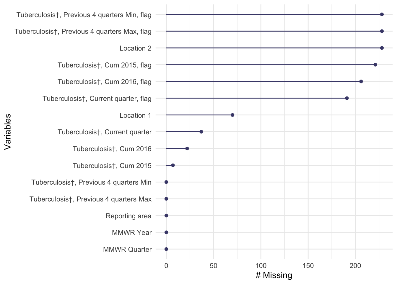
Describing the Variables
1. MMWR Quarter: This column indicates the quarter within the MMWR year to which the data corresponds. Quarters are often divided into four segments: 1 (January to March), 2 (April to June), 3 (July to September), and 4 (October to December).
Tuberculosis†, Cum 2016: This variable represents the cumulative number of tuberculosis cases reported up to the year 2016.
Tuberculosis†, Cum 2015: This variable represents the cumulative number of tuberculosis cases reported up to the year 2015.
Tuberculosis†, Previous 4 quarters Min: This column likely represents the minimum number of tuberculosis cases reported in the previous four quarters.
Tuberculosis†, Previous 4 quarters Max: This column likely represents the maximum number of tuberculosis cases reported in the previous four quarters.
# creating a new dataset from the above defined variable using subsetting and renaming the variables

# Subset and rename variables
newtb_data <- tb_data %>%
  subset(select = c("MMWR Quarter",
                     "Tuberculosis†, Previous 4 quarters Min",
                     "Tuberculosis†, Previous 4 quarters Max",
                     "Tuberculosis†, Cum 2016",
                     "Tuberculosis†, Cum 2015")) %>%
  rename(
    "mmwr_quarter" = "MMWR Quarter",
    "tb_prev_4_q_min" = "Tuberculosis†, Previous 4 quarters Min",
    "tb_prev_4_q_max" = "Tuberculosis†, Previous 4 quarters Max",
    "tbcases_2016" = "Tuberculosis†, Cum 2016",
    "tbcases_2015" = "Tuberculosis†, Cum 2015"
  )


# Display the first few rows of the new data frame (newtb_data)
head(newtb_data)
# A tibble: 6 × 5
mmwr_quarter tb_prev_4_q_min tb_prev_4_q_max tbcases_2016 tbcases_2015
<dbl> <dbl> <dbl> <dbl> <dbl>
1 1 40 90 40 41
2 1 4 24 4 9
3 1 3 7 5 1
4 1 28 56 28 26
5 1 0 4 NA 2
6 1 3 13 3 1#Looking at column names
colnames(tb_data) [1] "Reporting area"
[2] "MMWR Year"
[3] "MMWR Quarter"
[4] "Tuberculosis†, Current quarter"
[5] "Tuberculosis†, Current quarter, flag"
[6] "Tuberculosis†, Previous 4 quarters Min"
[7] "Tuberculosis†, Previous 4 quarters Min, flag"
[8] "Tuberculosis†, Previous 4 quarters Max"
[9] "Tuberculosis†, Previous 4 quarters Max, flag"
[10] "Tuberculosis†, Cum 2016"
[11] "Tuberculosis†, Cum 2016, flag"
[12] "Tuberculosis†, Cum 2015"
[13] "Tuberculosis†, Cum 2015, flag"
[14] "Location 1"
[15] "Location 2" ##Now looking at the missings in the newdata
# Visualize missing values for each variable using gg_miss_var from naniar package
naniar::gg_miss_var(newtb_data)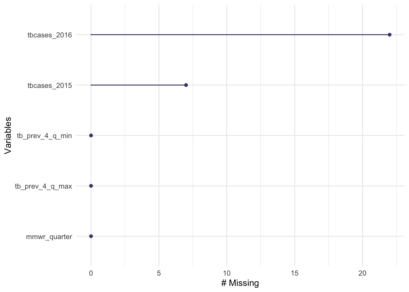
# Looking at the structure of the newtb_data
str(newtb_data)
tibble [228 × 5] (S3: tbl_df/tbl/data.frame)
$ mmwr_quarter : num [1:228] 1 1 1 1 1 1 1 1 1 1 ...
$ tb_prev_4_q_min: num [1:228] 40 4 3 28 0 3 0 38 31 25 ...
$ tb_prev_4_q_max: num [1:228] 90 24 7 56 4 13 2 118 63 61 ...
$ tbcases_2016 : num [1:228] 40 4 5 28 NA 3 NA 38 31 25 ...
$ tbcases_2015 : num [1:228] 41 9 1 26 2 1 2 20 23 26 ...# Convert mmwr_quarter to factor
newtb_data$mmwr_quarter <- as.factor(newtb_data$mmwr_quarter)
str(newtb_data)tibble [228 × 5] (S3: tbl_df/tbl/data.frame)
$ mmwr_quarter : Factor w/ 4 levels "1","2","3","4": 1 1 1 1 1 1 1 1 1 1 ...
$ tb_prev_4_q_min: num [1:228] 40 4 3 28 0 3 0 38 31 25 ...
$ tb_prev_4_q_max: num [1:228] 90 24 7 56 4 13 2 118 63 61 ...
$ tbcases_2016 : num [1:228] 40 4 5 28 NA 3 NA 38 31 25 ...
$ tbcases_2015 : num [1:228] 41 9 1 26 2 1 2 20 23 26 ...Visualization
# Load necessary libraries
library(ggplot2)  # for creating plots


# Create histograms for each variable
histograms <- list(
  # Histogram for Tuberculosis Previous 4 Quarters Min
  ggplot(newtb_data, aes(x = tb_prev_4_q_min)) +
    geom_histogram(fill = "blue", color = "black", bins = 20) +
    labs(x = "Tuberculosis Previous 4 Quarters Min", y = "Frequency",
         title = "Histogram of Tuberculosis Previous 4 Quarters Min"),

  # Histogram for Tuberculosis Previous 4 Quarters Max
  ggplot(newtb_data, aes(x = tb_prev_4_q_max)) +
    geom_histogram(fill = "blue", color = "black", bins = 20) +
    labs(x = "Tuberculosis Previous 4 Quarters Max", y = "Frequency",
         title = "Histogram of Tuberculosis Previous 4 Quarters Max"),

  # Histogram for Tuberculosis Cases 2016
  ggplot(newtb_data, aes(x = tbcases_2016)) +
    geom_histogram(fill = "blue", color = "black", bins = 20) +
    labs(x = "Tuberculosis Cases 2016", y = "Frequency",
         title = "Histogram of Tuberculosis Cases 2016"),

  # Histogram for Tuberculosis Cases 2015
  ggplot(newtb_data, aes(x = tbcases_2015)) +
    geom_histogram(fill = "blue", color = "black", bins = 20) +
    labs(x = "Tuberculosis Cases 2015", y = "Frequency",
         title = "Histogram of Tuberculosis Cases 2015")
)

# Display histograms side by side
grid.arrange(grobs = histograms, ncol = 2)
Warning: Removed 22 rows containing non-finite values (`stat_bin()`).Warning: Removed 7 rows containing non-finite values (`stat_bin()`).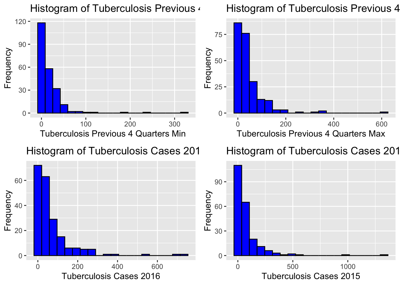
# Create a box plot of Tuberculosis Previous 4 Quarters Min by MMWR Quarter
ggplot(newtb_data, aes(x = factor(mmwr_quarter), y = tb_prev_4_q_min, fill = factor(mmwr_quarter))) +

  # Add a box plot layer with dodged position
  geom_boxplot(position = position_dodge(width = 0.8)) +

  # Label the x-axis as "MMWR Quarter" and y-axis as "Tuberculosis Previous 4 Quarters Min"
  labs(x = "MMWR Quarter", y = "Tuberculosis Previous 4 Quarters Min",
       title = "Box Plot of Tuberculosis Previous 4 Quarters Min by MMWR Quarter")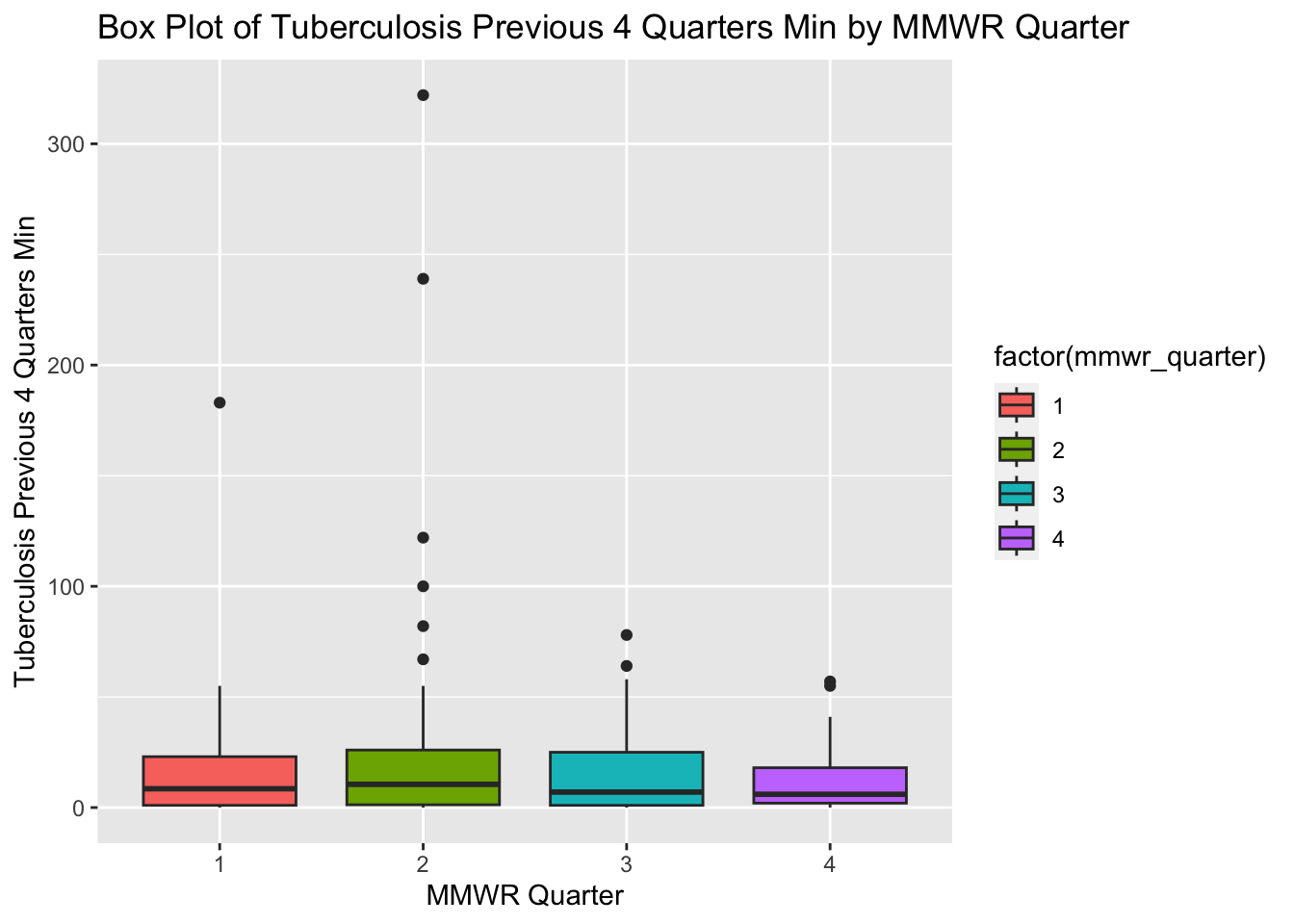
  # Create a box plot of Tuberculosis Previous 4 Quarters Max by MMWR Quarter
ggplot(newtb_data, aes(x = factor(mmwr_quarter), y = tb_prev_4_q_max, fill = factor(mmwr_quarter))) +

  # Add a box plot layer with dodged position
  geom_boxplot(position = position_dodge(width = 10)) +

  # Label the x-axis as "MMWR Quarter" and y-axis as "Tuberculosis Previous 4 Quarters Max"
  labs(x = "MMWR Quarter", y = "Tuberculosis Previous 4 Quarters Max",
       title = "Box Plot of Tuberculosis Previous 4 Quarters Max by MMWR Quarter")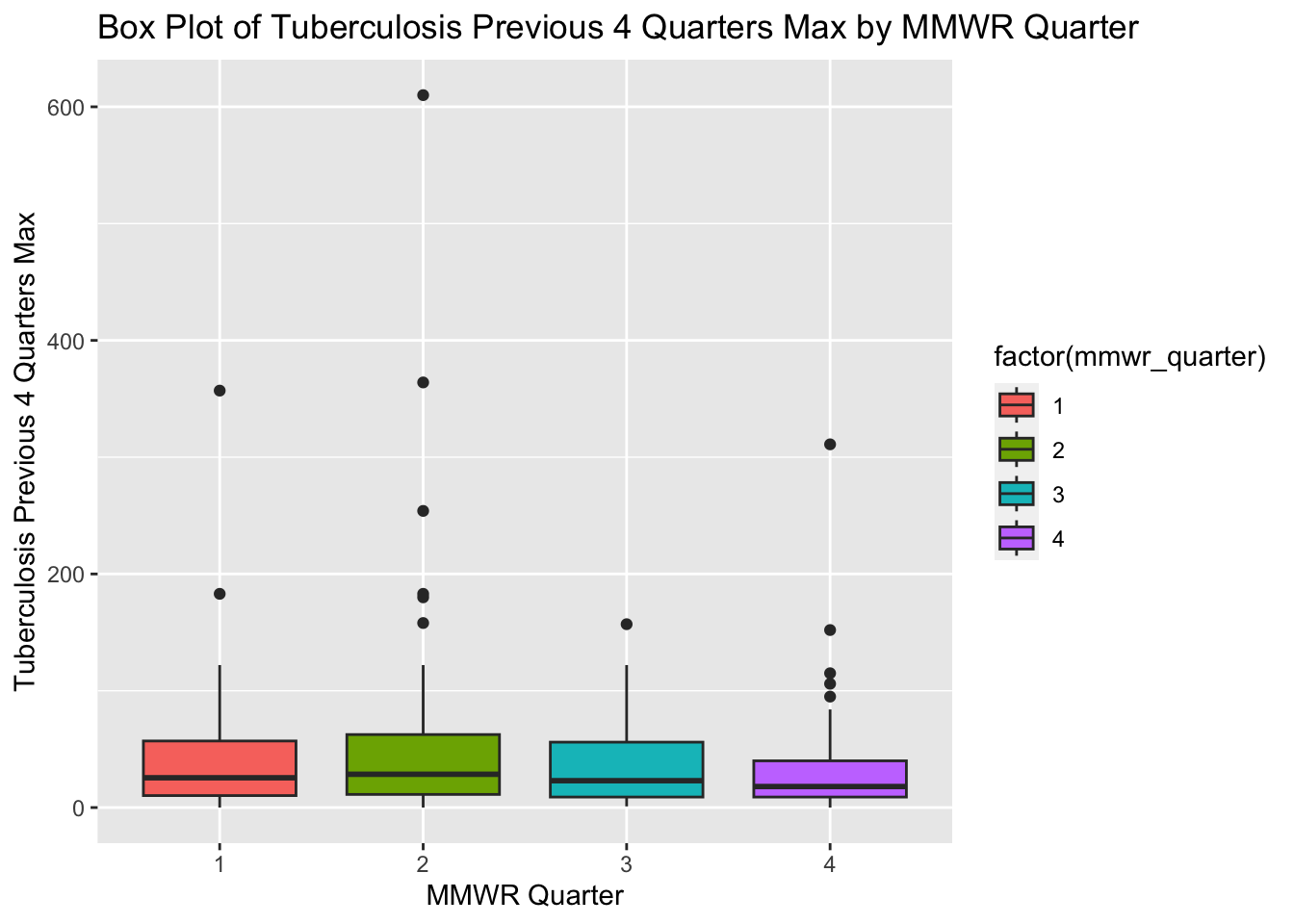
  # Create a box plot of Tuberculosis Cases 2016 by MMWR Quarter
ggplot(newtb_data, aes(x = factor(mmwr_quarter), y = tbcases_2016, fill = factor(mmwr_quarter))) +

  # Add a box plot layer with dodged position
  geom_boxplot(position = position_dodge(width = 10)) +

  # Label the x-axis as "MMWR Quarter" and y-axis as "Tuberculosis Cases 2016"
  labs(x = "MMWR Quarter", y = "Tuberculosis Cases 2016",
       title = "Box Plot of Tuberculosis Cases 2016 by MMWR Quarter")
Warning: Removed 22 rows containing non-finite values (`stat_boxplot()`).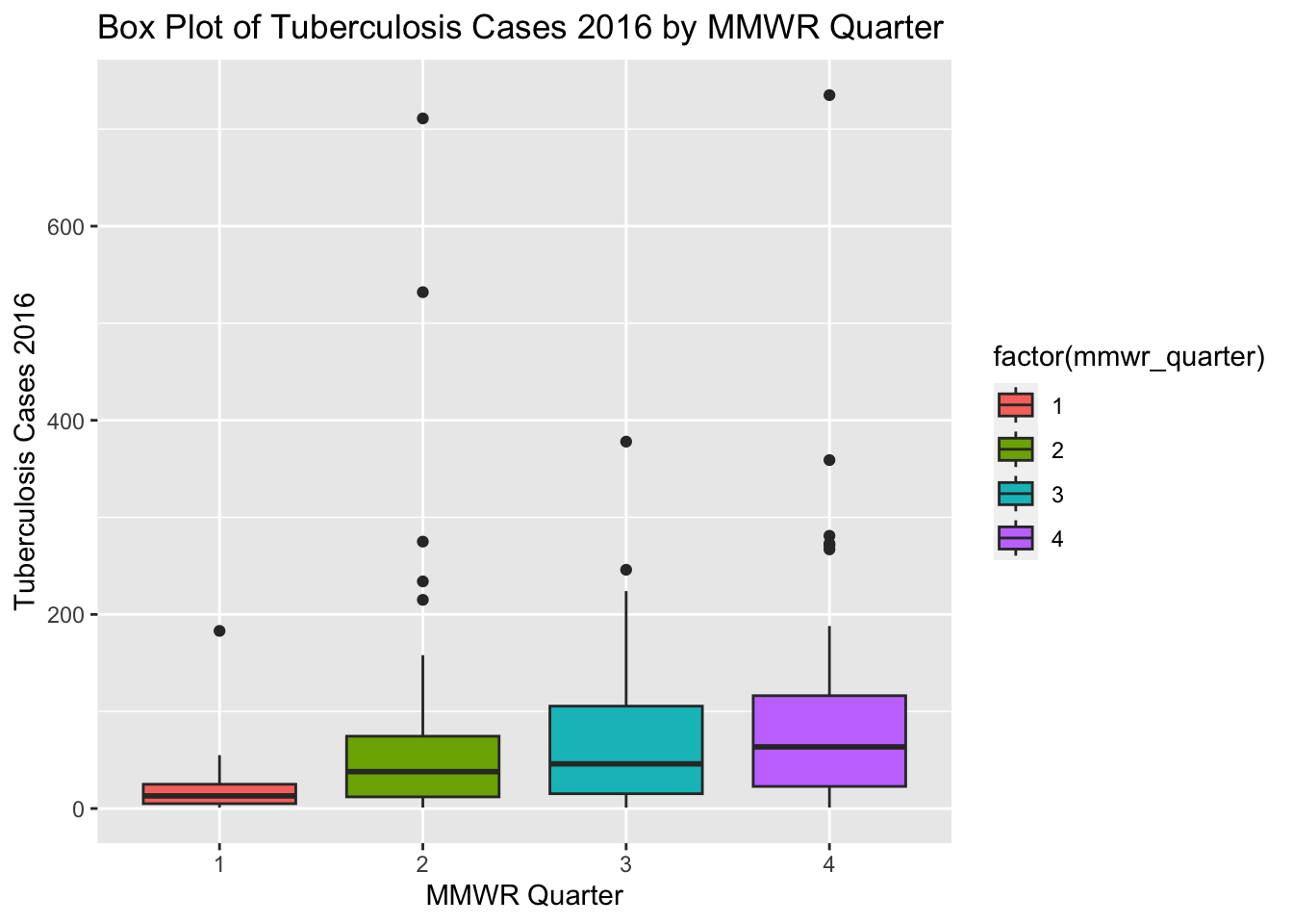
# Create a box plot of Tuberculosis Cases 2015 by MMWR Quarter
ggplot(newtb_data, aes(x = factor(mmwr_quarter), y = tbcases_2015, fill = factor(mmwr_quarter))) +

  # Add a box plot layer with dodged position
  geom_boxplot(position = position_dodge(width = 10)) +

  # Label the x-axis as "MMWR Quarter" and y-axis as "Tuberculosis Cases 2015"
  labs(x = "MMWR Quarter", y = "Tuberculosis Cases 2015",
       title = "Box Plot of Tuberculosis Cases 2015 by MMWR Quarter")
Warning: Removed 7 rows containing non-finite values (`stat_boxplot()`).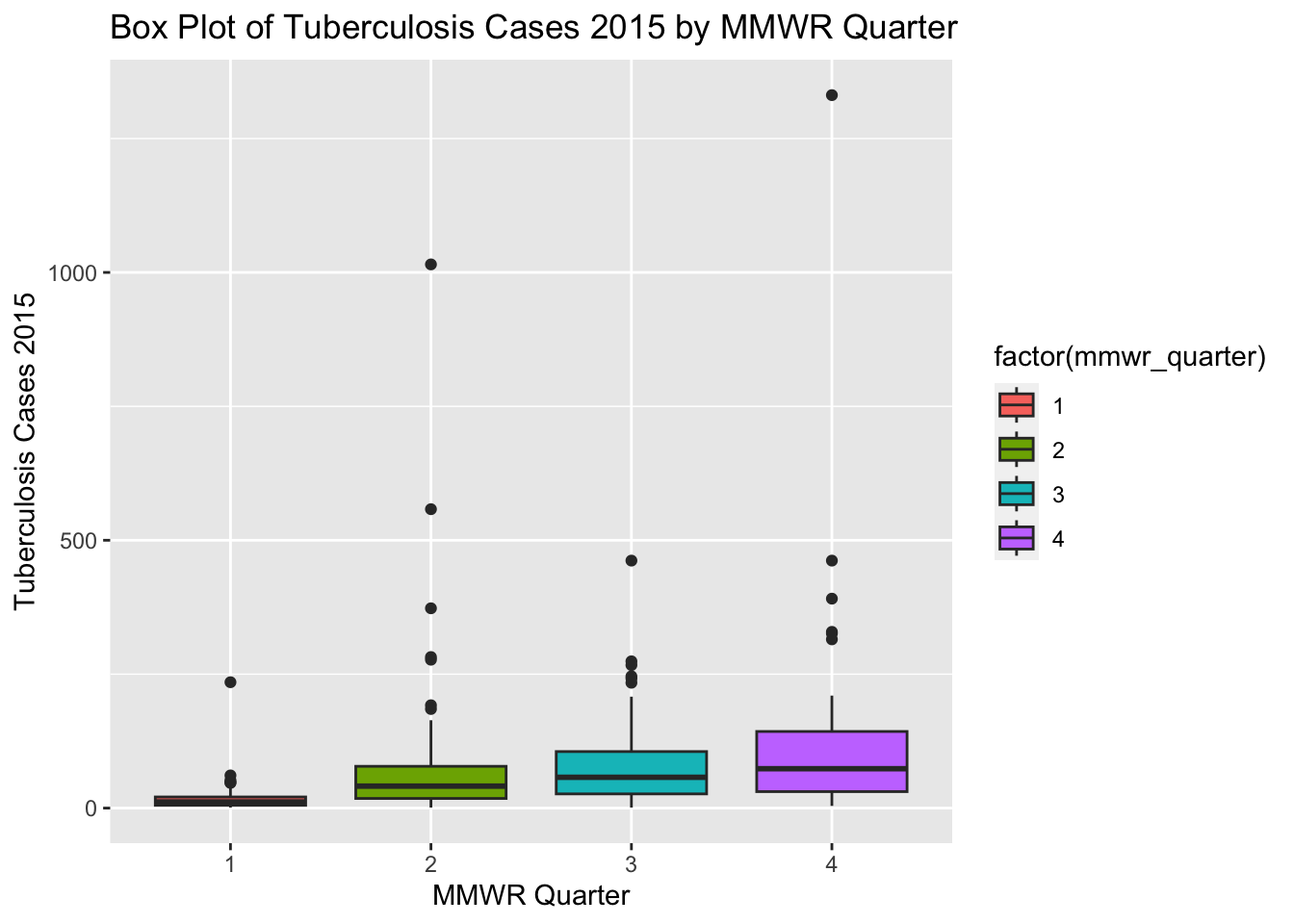
Data Summary
summary(newtb_data) mmwr_quarter tb_prev_4_q_min tb_prev_4_q_max tbcases_2016
1:58 Min. : 0.00 Min. : 0.00 Min. : 1.00
2:62 1st Qu.: 1.00 1st Qu.: 10.00 1st Qu.: 12.00
3:57 Median : 8.00 Median : 24.00 Median : 33.00
4:51 Mean : 18.15 Mean : 44.82 Mean : 67.33
3rd Qu.: 25.00 3rd Qu.: 57.00 3rd Qu.: 79.00
Max. :322.00 Max. :610.00 Max. :735.00
NA's :22
tbcases_2015
Min. : 1.00
1st Qu.: 12.00
Median : 36.00
Mean : 80.31
3rd Qu.: 90.00
Max. :1331.00
NA's :7 This section is contributed by Ranni Tewfik.
Part 1 - Generating the Synthetic Dataset
#Explore the five variables in the original processed data
table(newtb_data$mmwr_quarter)
 1  2  3  4
58 62 57 51 summary(newtb_data$tb_prev_4_q_min) Min. 1st Qu. Median Mean 3rd Qu. Max.
0.00 1.00 8.00 18.15 25.00 322.00 summary(newtb_data$tb_prev_4_q_max) Min. 1st Qu. Median Mean 3rd Qu. Max.
0.00 10.00 24.00 44.82 57.00 610.00 summary(newtb_data$tbcases_2016) Min. 1st Qu. Median Mean 3rd Qu. Max. NA's
1.00 12.00 33.00 67.33 79.00 735.00 22 summary(newtb_data$tbcases_2015) Min. 1st Qu. Median Mean 3rd Qu. Max. NA's
1.00 12.00 36.00 80.31 90.00 1331.00 7 #Load required R package
library(dplyr)
#Set seed for reproducibility
set.seed(123)
#Define number of individuals for each mmwr_quarter level
mmwr_quarter_levels <- c(rep(1, 58), rep(2, 62), rep(3, 57), rep(4, 51))
#Generate mmwr_quarter variable
mmwr_quarter <- factor(sample(mmwr_quarter_levels))
#Generate other variables based on specified distributions
tb_prev_4_q_min <- round(rnorm(228, mean = 18.15, sd = 10))
tb_prev_4_q_min <- pmax(tb_prev_4_q_min, 0)
tb_prev_4_q_max <- round(rnorm(228, mean = 44.82, sd = 20))
tb_prev_4_q_max <- pmax(tb_prev_4_q_max, 0)
tb_cases_2016 <- round(rnorm(228, mean = 67.33, sd = 50))
tb_cases_2016 <- pmax(tb_cases_2016, 1)
tb_cases_2016[sample(1:228, 22)] <- NA
tb_cases_2015 <- round(rnorm(228, mean = 80.31, sd = 60))
tb_cases_2015 <- pmax(tb_cases_2015, 1)
tb_cases_2015[sample(1:228, 7)] <- NA
#Create the synthetic dataset
newtb_data_rt <- data.frame(
mmwr_quarter = mmwr_quarter,
tb_prev_4_q_min = tb_prev_4_q_min,
tb_prev_4_q_max = tb_prev_4_q_max,
tb_cases_2016 = tb_cases_2016,
tb_cases_2015 = tb_cases_2015)
#Get an overview and summary of the data
str(newtb_data_rt)'data.frame': 228 obs. of 5 variables:
$ mmwr_quarter : Factor w/ 4 levels "1","2","3","4": 3 4 4 1 4 3 1 2 1 4 ...
$ tb_prev_4_q_min: num 14 29 8 6 51 14 21 25 13 23 ...
$ tb_prev_4_q_max: num 22 36 52 32 2 63 28 33 75 29 ...
$ tb_cases_2016 : num 1 45 34 6 145 1 83 110 76 24 ...
$ tb_cases_2015 : num 149 177 82 7 62 51 127 104 29 72 ...summary(newtb_data_rt) mmwr_quarter tb_prev_4_q_min tb_prev_4_q_max tb_cases_2016 tb_cases_2015
1:58 Min. : 0.00 Min. : 0.00 Min. : 1.00 Min. : 1.00
2:62 1st Qu.:12.00 1st Qu.:32.75 1st Qu.: 31.00 1st Qu.: 38.00
3:57 Median :18.00 Median :44.50 Median : 68.00 Median : 79.00
4:51 Mean :18.79 Mean :44.89 Mean : 68.55 Mean : 82.16
3rd Qu.:25.00 3rd Qu.:58.25 3rd Qu.: 99.00 3rd Qu.:123.00
Max. :51.00 Max. :93.00 Max. :202.00 Max. :242.00
NA's :22 NA's :7 First, I explored the original processed dataset “newtb_data” to better understand the variables and their distributions. I used ChatGPT to help me produce the synthetic dataset “newtb_data_rt” with the same structure as “newtb_data”.
ChatGPT prompt:
“Write R code that generates a dataset of 228 individuals with five variables: mmwr_quarter, tb_prev_4_q_min, tb_prev_4_q_max, tbcases_2016, and tbcases_2015. The variable mmwr_quarter is a factor variable and has four levels: level 1 with 58 individuals, level 2 with 62 individuals, level 3 with 57 individuals, and level 4 with 51 individuals. The variable tb_prev_4_q_min is numerical with whole integers ranging from 0 to 322, median is 8, and mean is 18.15. The variable tb_prev_4_q_max is numerical with whole integers ranging from 0 to 610, median is 24, and mean is 44.82. The variable tb_cases_2016 is numerical with whole integers ranging from 1 to 735, median is 33, mean is 67.33, and 22 individuals with missing value. The variable tb_cases_2015 is numerical with whole integers ranging from 1 to 1331, median is 36, mean is 80.31, and 7 individuals with missing value. Add thorough documentation to the R code.”
Part 2 - Exploring the Synthetic Dataset
# Create histograms for each variable
histograms <- list(
  # Histogram for Tuberculosis Previous 4 Quarters Min
  ggplot(newtb_data_rt, aes(x = tb_prev_4_q_min)) +
    geom_histogram(fill = "blue", color = "black", bins = 20) +
    labs(x = "Tuberculosis Previous 4 Quarters Min", y = "Frequency",
         title = "Histogram of Tuberculosis Previous 4 Quarters Min"),

  # Histogram for Tuberculosis Previous 4 Quarters Max
  ggplot(newtb_data_rt, aes(x = tb_prev_4_q_max)) +
    geom_histogram(fill = "blue", color = "black", bins = 20) +
    labs(x = "Tuberculosis Previous 4 Quarters Max", y = "Frequency",
         title = "Histogram of Tuberculosis Previous 4 Quarters Max"),

  # Histogram for Tuberculosis Cases 2016
  ggplot(newtb_data_rt, aes(x = tb_cases_2016)) +
    geom_histogram(fill = "blue", color = "black", bins = 20) +
    labs(x = "Tuberculosis Cases 2016", y = "Frequency",
         title = "Histogram of Tuberculosis Cases 2016"),

  # Histogram for Tuberculosis Cases 2015
  ggplot(newtb_data_rt, aes(x = tb_cases_2015)) +
    geom_histogram(fill = "blue", color = "black", bins = 20) +
    labs(x = "Tuberculosis Cases 2015", y = "Frequency",
         title = "Histogram of Tuberculosis Cases 2015")
)

# Display histograms side by side
grid.arrange(grobs = histograms, ncol = 2)
Warning: Removed 22 rows containing non-finite values (`stat_bin()`).Warning: Removed 7 rows containing non-finite values (`stat_bin()`).
The histograms for the variables “tb_prev_4_q_min” and “tb_prev_4_q_max” show an approximately normal distribution, but the histograms for the variables “tb_cases_2016” and “tb_cases_2015” do not show an approximately normal distribution. The histograms in the new synthetic dataset look slightly similar to the histograms in the original processed dataset for the variables “tb_cases_2016” and “tb_cases_2015” but not for the variables “tb_prev_4_q_min” and “tb_prev_4_q_max”.
# Create a box plot of Tuberculosis Previous 4 Quarters Min by MMWR Quarter
ggplot(newtb_data_rt, aes(x = factor(mmwr_quarter), y = tb_prev_4_q_min, fill = factor(mmwr_quarter))) +

  # Add a box plot layer with dodged position
  geom_boxplot(position = position_dodge(width = 0.8)) +

  # Label the x-axis as "MMWR Quarter" and y-axis as "Tuberculosis Previous 4 Quarters Min"
  labs(x = "MMWR Quarter", y = "Tuberculosis Previous 4 Quarters Min",
       title = "Box Plot of Tuberculosis Previous 4 Quarters Min by MMWR Quarter")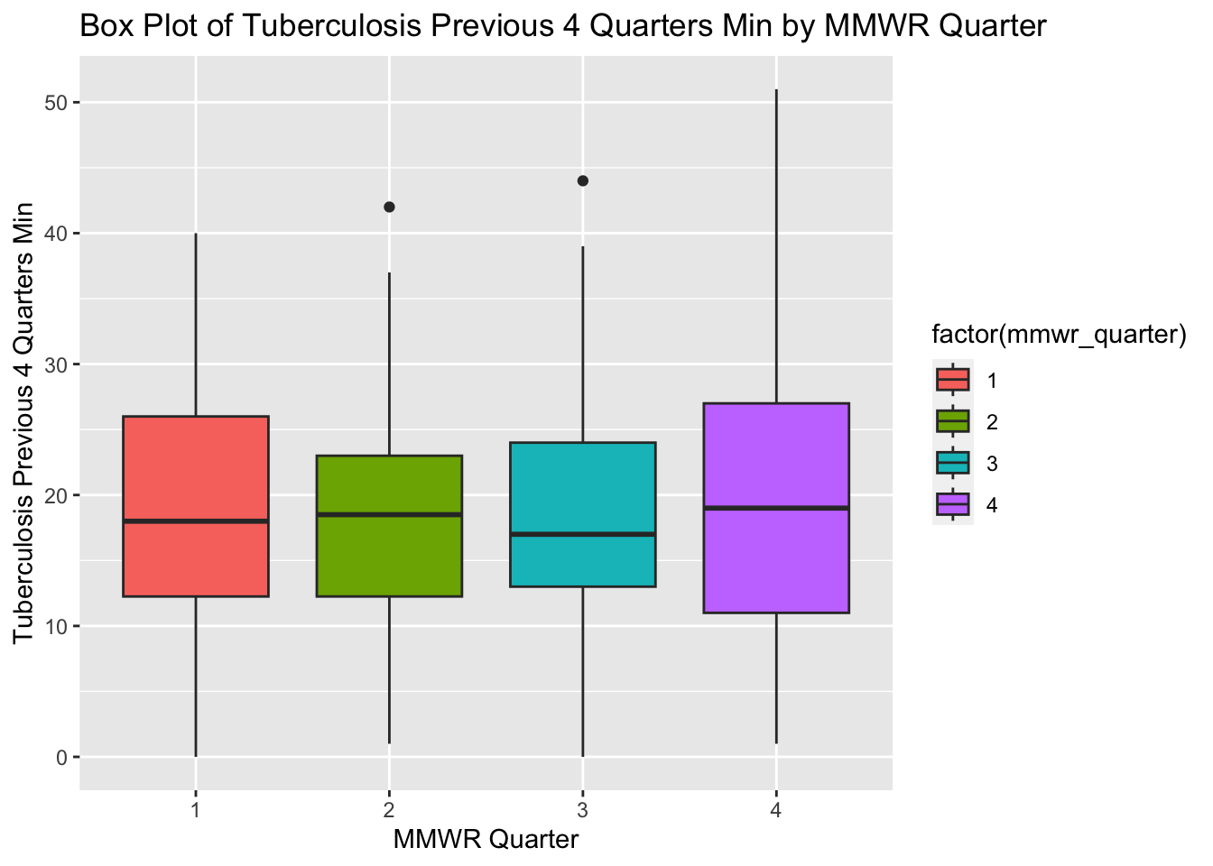
The box plots for tuberculosis for the previous four MMWR quarters (min) show an approximately normal distribution, however, MMWR Quarters 3 and 4 are slightly positively skewed. The box plots in the original processed dataset have more positive skew and more outliers compared with the box plots in the new synthetic data set.
  # Create a box plot of Tuberculosis Previous 4 Quarters Max by MMWR Quarter
ggplot(newtb_data_rt, aes(x = factor(mmwr_quarter), y = tb_prev_4_q_max, fill = factor(mmwr_quarter))) +

  # Add a box plot layer with dodged position
  geom_boxplot(position = position_dodge(width = 10)) +

  # Label the x-axis as "MMWR Quarter" and y-axis as "Tuberculosis Previous 4 Quarters Max"
  labs(x = "MMWR Quarter", y = "Tuberculosis Previous 4 Quarters Max",
       title = "Box Plot of Tuberculosis Previous 4 Quarters Max by MMWR Quarter")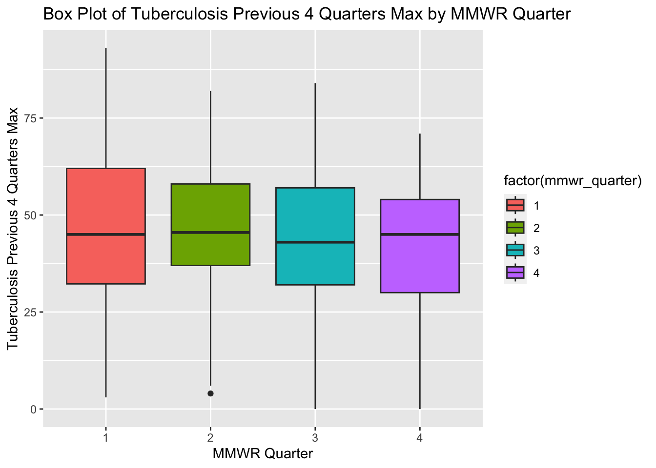
The box plots for tuberculosis for the previous four MMWR quarters (max) show an approximately normal distribution. The box plots in the original processed dataset have more positive skew and more outliers compared with the box plots in the new synthetic data set.
  # Create a box plot of Tuberculosis Cases 2016 by MMWR Quarter
ggplot(newtb_data_rt, aes(x = factor(mmwr_quarter), y = tb_cases_2016, fill = factor(mmwr_quarter))) +

  # Add a box plot layer with dodged position
  geom_boxplot(position = position_dodge(width = 10)) +

  # Label the x-axis as "MMWR Quarter" and y-axis as "Tuberculosis Cases 2016"
  labs(x = "MMWR Quarter", y = "Tuberculosis Cases 2016",
       title = "Box Plot of Tuberculosis Cases 2016 by MMWR Quarter")
Warning: Removed 22 rows containing non-finite values (`stat_boxplot()`).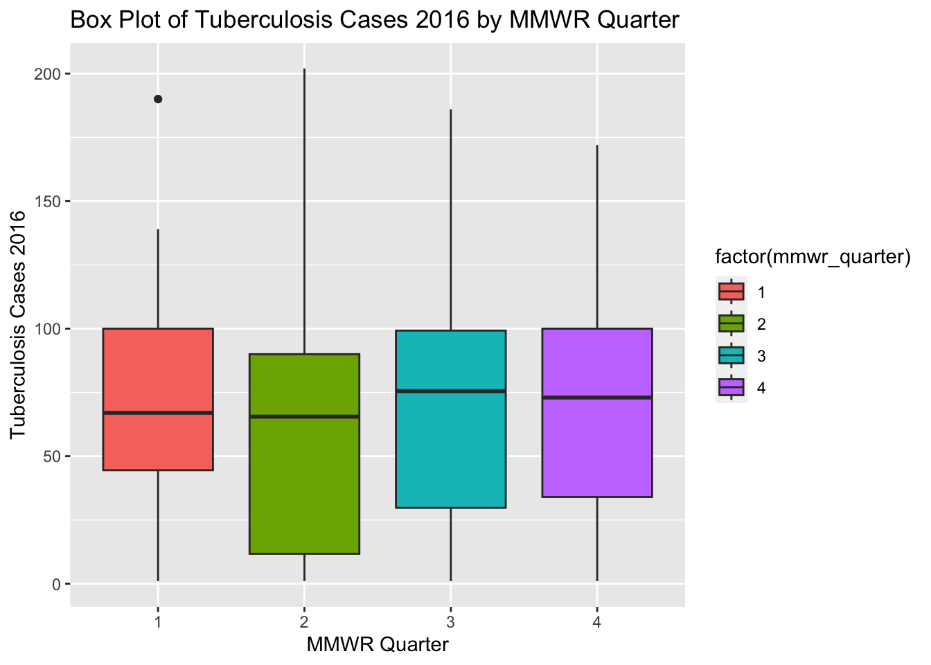
The box plots for tuberculosis cases in 2016 for different MMWR quarters are positively skewed with some outliers. The box plots in the new synthetic dataset are somewhat similar to the box plots in the original processed dataset.
# Create a box plot of Tuberculosis Cases 2015 by MMWR Quarter
ggplot(newtb_data_rt, aes(x = factor(mmwr_quarter), y = tb_cases_2015, fill = factor(mmwr_quarter))) +

  # Add a box plot layer with dodged position
  geom_boxplot(position = position_dodge(width = 10)) +

  # Label the x-axis as "MMWR Quarter" and y-axis as "Tuberculosis Cases 2015"
  labs(x = "MMWR Quarter", y = "Tuberculosis Cases 2015",
       title = "Box Plot of Tuberculosis Cases 2015 by MMWR Quarter")
Warning: Removed 7 rows containing non-finite values (`stat_boxplot()`).
The box plots for tuberculosis cases in 2015 for different MMWR quarters show an approximate normal distribution. The box plots in the new synthetic dataset are not similar to the box plots in the original processed dataset.