| skim_type | skim_variable | n_missing | complete_rate | character.min | character.max | character.empty | character.n_unique | character.whitespace | factor.ordered | factor.n_unique | factor.top_counts | numeric.mean | numeric.sd | numeric.p0 | numeric.p25 | numeric.p50 | numeric.p75 | numeric.p100 | numeric.hist |
|---|---|---|---|---|---|---|---|---|---|---|---|---|---|---|---|---|---|---|---|
| character | Educ | 0 | 1 | 7 | 13 | 0 | 4 | 0 | NA | NA | NA | NA | NA | NA | NA | NA | NA | NA | NA |
| factor | Gender | 0 | 1 | NA | NA | NA | NA | NA | FALSE | 3 | M: 4, F: 3, O: 2 | NA | NA | NA | NA | NA | NA | NA | NA |
| numeric | Height | 0 | 1 | NA | NA | NA | NA | NA | NA | NA | NA | 165.66667 | 15.97655 | 133 | 156 | 166 | 178 | 183 | ▂▁▃▃▇ |
| numeric | Weight | 0 | 1 | NA | NA | NA | NA | NA | NA | NA | NA | 70.11111 | 21.24526 | 45 | 55 | 70 | 80 | 110 | ▇▂▃▂▂ |
| numeric | age | 0 | 1 | NA | NA | NA | NA | NA | NA | NA | NA | 41.66667 | 13.39776 | 22 | 34 | 45 | 54 | 56 | ▃▂▂▂▇ |
MADA Data Analysis Project
Jayne Musso contributed to this exercise
1 Summary/Abstract
Write a summary of your project.
2 Introduction
2.1 General Background Information
Provide enough background on your topic that others can understand the why and how of your analysis
2.2 Description of data and data source
Describe what the data is, what it contains, where it is from, etc. Eventually this might be part of a methods section.
2.3 Questions/Hypotheses to be addressed
3 Methods
Describe your methods. That should describe the data, the cleaning processes, and the analysis approaches. You might want to provide a shorter description here and all the details in the supplement.
3.1 Data aquisition
3.2 Data import and cleaning
3.3 Statistical analysis
Explain anything related to your statistical analyses.
4 Results
4.1 Exploratory/Descriptive analysis
4.2 Basic statistical analysis
Figure1: shows a scatterplot figure produced by one of the R scripts.
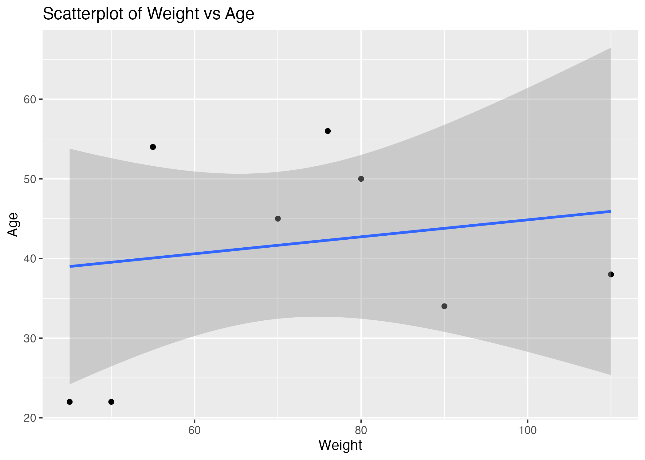
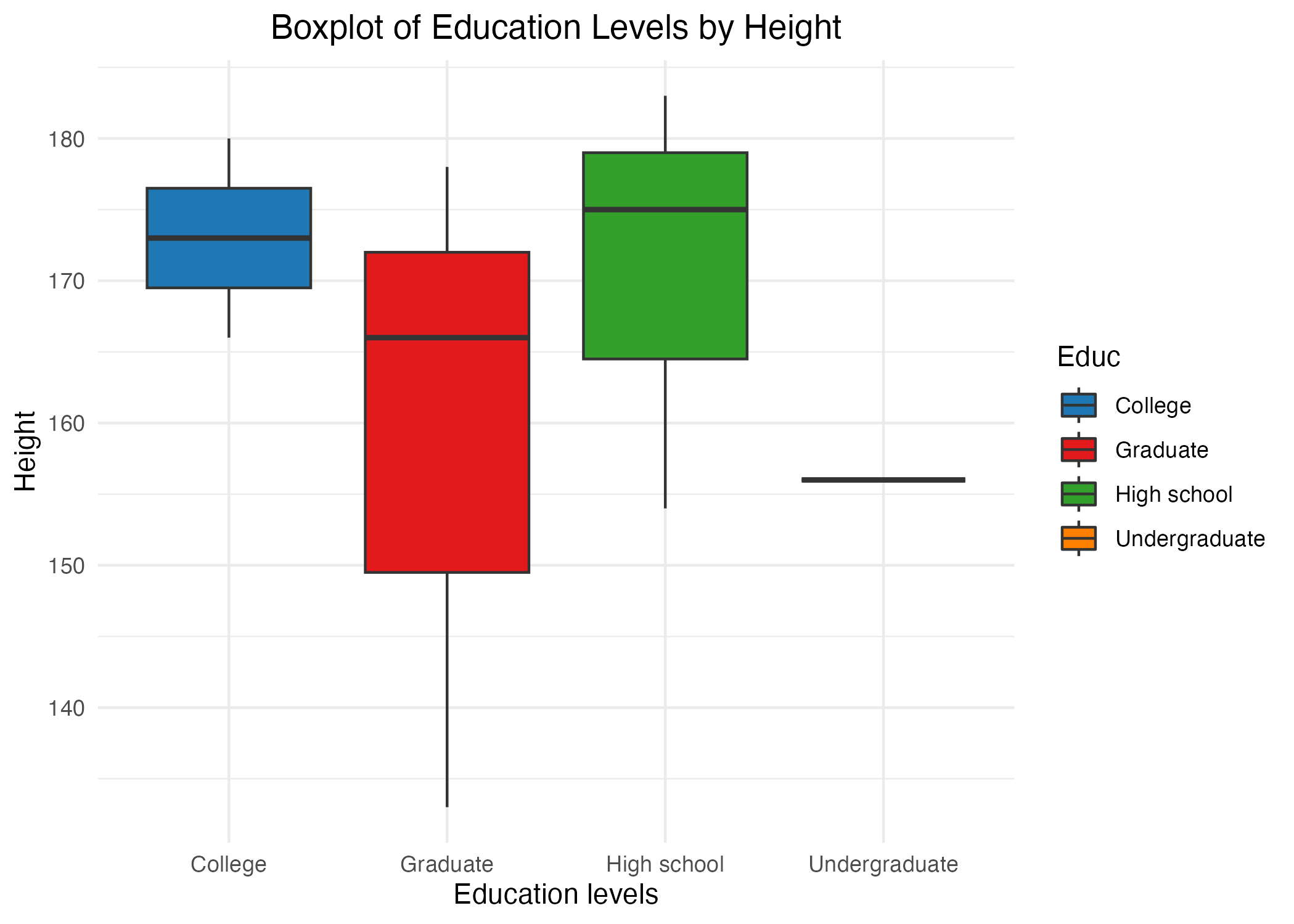
Figure2: shows a Boxplot of Height and Education Levels.
4.3 Full analysis
Table2: shows a summary of a linear model fit .
| term | estimate | std.error | statistic | p.value |
|---|---|---|---|---|
| (Intercept) | 116.7253978 | 14.9101494 | 7.8285867 | 0.0014375 |
| age | 1.0822039 | 0.2607536 | 4.1502937 | 0.0142569 |
| EducGraduate | 0.4293852 | 8.7286474 | 0.0491926 | 0.9631241 |
| EducHigh school | 10.2923787 | 8.5648274 | 1.2017030 | 0.2957598 |
| EducUndergraduate | 2.4796700 | 11.7223156 | 0.2115341 | 0.8428112 |
4.4 Code used for the analysis
##############################################
### Box Plot
b1<-mydata %>%
  ggplot(mapping = aes(x = `Educ`, y = Height, fill = `Educ`)) +
  geom_boxplot() +
  scale_fill_manual(values = c("College" = "#1f78b4", "High school" = "#33a02c", "Graduate" = "#e31a1c", "Undergraduate" = "#ff7f00")) +
  theme_minimal() +
  labs(x = "Education levels", y = "Height") +
  ggtitle("Boxplot of Education Levels by Height") +
  theme(plot.title = element_text(hjust = 0.5))  # Adjust title alignment
b1
figure_file = here("starter-analysis-exercise","results","figures","education-Height-stratified.png")
ggsave(filename = figure_file, plot=b1)
##############################################
For the scatter Plot
s1 <- ggplot(mydata, aes(x = Weight, y = age)) +
  geom_point() +
  stat_smooth(method = "glm", formula = y ~ x) +
  ggtitle("Scatterplot of Weight vs Age") +
  labs(x = "Weight", y = "Age")
s1
figure_file = here("starter-analysis-exercise","results","figures","Weight-Age-stratified.png")
ggsave(filename = figure_file, plot=s1)

############################
#### Third model fit
# fit linear model using height as outcome, age and Educatinal Levels as predictor

lmfit3 <- lm(Height ~ age + Educ, mydata)

# place results from fit into a data frame with the tidy function
lmtable3 <- broom::tidy(lmfit3)

#look at fit results
print(lmtable3)

# save fit results table
table_file3 = here("starter-analysis-exercise","results", "tables-files", "resulttable3.rds")
saveRDS(lmtable3, file = table_file3)
5 Discussion
5.1 Summary and Interpretation
Summarize what you did, what you found and what it means.
5.2 Strengths and Limitations
Discuss what you perceive as strengths and limitations of your analysis.
5.3 Conclusions
What are the main take-home messages?
Include citations in your Rmd file using bibtex, the list of references will automatically be placed at the end
This paper (Leek & Peng, 2015) discusses types of analyses.
These papers (McKay, Ebell, Billings, et al., 2020; McKay, Ebell, Dale, Shen, & Handel, 2020) are good examples of papers published using a fully reproducible setup similar to the one shown in this template.
6 References
Leek, J. T., & Peng, R. D. (2015). Statistics. What is the question? Science (New York, N.Y.), 347(6228), 1314–1315. https://doi.org/10.1126/science.aaa6146
McKay, B., Ebell, M., Billings, W. Z., Dale, A. P., Shen, Y., & Handel, A. (2020). Associations Between Relative Viral Load at Diagnosis and Influenza A Symptoms and Recovery. Open Forum Infectious Diseases, 7(11), ofaa494. https://doi.org/10.1093/ofid/ofaa494
McKay, B., Ebell, M., Dale, A. P., Shen, Y., & Handel, A. (2020). Virulence-mediated infectiousness and activity trade-offs and their impact on transmission potential of influenza patients. Proceedings. Biological Sciences, 287(1927), 20200496. https://doi.org/10.1098/rspb.2020.0496