R Coding Exercise

Loading and checking data

#loading packages
library(dslabs)
library(tidyverse)

── Attaching core tidyverse packages ──────────────────────── tidyverse 2.0.0 ──
✔ dplyr     1.1.4     ✔ readr     2.1.4
✔ forcats   1.0.0     ✔ stringr   1.5.1
✔ ggplot2   3.4.4     ✔ tibble    3.2.1
✔ lubridate 1.9.3     ✔ tidyr     1.3.0
✔ purrr     1.0.2     
── Conflicts ────────────────────────────────────────── tidyverse_conflicts() ──
✖ dplyr::filter() masks stats::filter()
✖ dplyr::lag()    masks stats::lag()
ℹ Use the conflicted package (<http://conflicted.r-lib.org/>) to force all conflicts to become errors

library(dplyr)
library(ggplot2)
library(ggthemes)
head(gapminder)

              country year infant_mortality life_expectancy fertility
1             Albania 1960           115.40           62.87      6.19
2             Algeria 1960           148.20           47.50      7.65
3              Angola 1960           208.00           35.98      7.32
4 Antigua and Barbuda 1960               NA           62.97      4.43
5           Argentina 1960            59.87           65.39      3.11
6             Armenia 1960               NA           66.86      4.55
  population          gdp continent          region
1    1636054           NA    Europe Southern Europe
2   11124892  13828152297    Africa Northern Africa
3    5270844           NA    Africa   Middle Africa
4      54681           NA  Americas       Caribbean
5   20619075 108322326649  Americas   South America
6    1867396           NA      Asia    Western Asia

Processing data

#get an overview of data structure
str(gapminder)

'data.frame':   10545 obs. of  9 variables:
 $ country         : Factor w/ 185 levels "Albania","Algeria",..: 1 2 3 4 5 6 7 8 9 10 ...
 $ year            : int  1960 1960 1960 1960 1960 1960 1960 1960 1960 1960 ...
 $ infant_mortality: num  115.4 148.2 208 NA 59.9 ...
 $ life_expectancy : num  62.9 47.5 36 63 65.4 ...
 $ fertility       : num  6.19 7.65 7.32 4.43 3.11 4.55 4.82 3.45 2.7 5.57 ...
 $ population      : num  1636054 11124892 5270844 54681 20619075 ...
 $ gdp             : num  NA 1.38e+10 NA NA 1.08e+11 ...
 $ continent       : Factor w/ 5 levels "Africa","Americas",..: 4 1 1 2 2 3 2 5 4 3 ...
 $ region          : Factor w/ 22 levels "Australia and New Zealand",..: 19 11 10 2 15 21 2 1 22 21 ...

#determine the type of object gapminder is
class(gapminder)

[1] "data.frame"

#  Code that assigns only the African countries to a new object/variable called africadata. 
#Run str and summary on the new object you created.

# Use subset to filter rows where Continent is "Africa"
africadata <- subset(gapminder, continent == "Africa")

# Display the structure of africadata
str(africadata)

'data.frame':   2907 obs. of  9 variables:
 $ country         : Factor w/ 185 levels "Albania","Algeria",..: 2 3 18 22 26 27 29 31 32 33 ...
 $ year            : int  1960 1960 1960 1960 1960 1960 1960 1960 1960 1960 ...
 $ infant_mortality: num  148 208 187 116 161 ...
 $ life_expectancy : num  47.5 36 38.3 50.3 35.2 ...
 $ fertility       : num  7.65 7.32 6.28 6.62 6.29 6.95 5.65 6.89 5.84 6.25 ...
 $ population      : num  11124892 5270844 2431620 524029 4829291 ...
 $ gdp             : num  1.38e+10 NA 6.22e+08 1.24e+08 5.97e+08 ...
 $ continent       : Factor w/ 5 levels "Africa","Americas",..: 1 1 1 1 1 1 1 1 1 1 ...
 $ region          : Factor w/ 22 levels "Australia and New Zealand",..: 11 10 20 17 20 5 10 20 10 10 ...

# Display summary statistics of africadata
summary(africadata)

         country          year      infant_mortality life_expectancy
 Algeria     :  57   Min.   :1960   Min.   : 11.40   Min.   :13.20  
 Angola      :  57   1st Qu.:1974   1st Qu.: 62.20   1st Qu.:48.23  
 Benin       :  57   Median :1988   Median : 93.40   Median :53.98  
 Botswana    :  57   Mean   :1988   Mean   : 95.12   Mean   :54.38  
 Burkina Faso:  57   3rd Qu.:2002   3rd Qu.:124.70   3rd Qu.:60.10  
 Burundi     :  57   Max.   :2016   Max.   :237.40   Max.   :77.60  
 (Other)     :2565                  NA's   :226                     
   fertility       population             gdp               continent   
 Min.   :1.500   Min.   :    41538   Min.   :4.659e+07   Africa  :2907  
 1st Qu.:5.160   1st Qu.:  1605232   1st Qu.:8.373e+08   Americas:   0  
 Median :6.160   Median :  5570982   Median :2.448e+09   Asia    :   0  
 Mean   :5.851   Mean   : 12235961   Mean   :9.346e+09   Europe  :   0  
 3rd Qu.:6.860   3rd Qu.: 13888152   3rd Qu.:6.552e+09   Oceania :   0  
 Max.   :8.450   Max.   :182201962   Max.   :1.935e+11                  
 NA's   :51      NA's   :51          NA's   :637                        
                       region   
 Eastern Africa           :912  
 Western Africa           :912  
 Middle Africa            :456  
 Northern Africa          :342  
 Southern Africa          :285  
 Australia and New Zealand:  0  
 (Other)                  :  0

#Take the africadata object and create two new objects (name them whatever you want),
#one that contains only infant_mortality and life_expectancy and one that contains 
#only population and life_expectancy.

# Assuming africadata has columns like "infant_mortality," "life_expectancy," and "population"
# Replace column names as per your actual data frame structure


# Create object with only "infant_mortality" and "life_expectancy"
subset1 <- select(africadata, infant_mortality, life_expectancy)

# Create object with only "population" and "life_expectancy"
subset2 <- select(africadata, population, life_expectancy)

# Display the structure of subset1 and subset1
str(subset1)

'data.frame':   2907 obs. of  2 variables:
 $ infant_mortality: num  148 208 187 116 161 ...
 $ life_expectancy : num  47.5 36 38.3 50.3 35.2 ...

str(subset2)

'data.frame':   2907 obs. of  2 variables:
 $ population     : num  11124892 5270844 2431620 524029 4829291 ...
 $ life_expectancy: num  47.5 36 38.3 50.3 35.2 ...

# Display summary statistics of subset1
summary(subset1)

 infant_mortality life_expectancy
 Min.   : 11.40   Min.   :13.20  
 1st Qu.: 62.20   1st Qu.:48.23  
 Median : 93.40   Median :53.98  
 Mean   : 95.12   Mean   :54.38  
 3rd Qu.:124.70   3rd Qu.:60.10  
 Max.   :237.40   Max.   :77.60  
 NA's   :226

summary(subset2)

   population        life_expectancy
 Min.   :    41538   Min.   :13.20  
 1st Qu.:  1605232   1st Qu.:48.23  
 Median :  5570982   Median :53.98  
 Mean   : 12235961   Mean   :54.38  
 3rd Qu.: 13888152   3rd Qu.:60.10  
 Max.   :182201962   Max.   :77.60  
 NA's   :51

Plotting

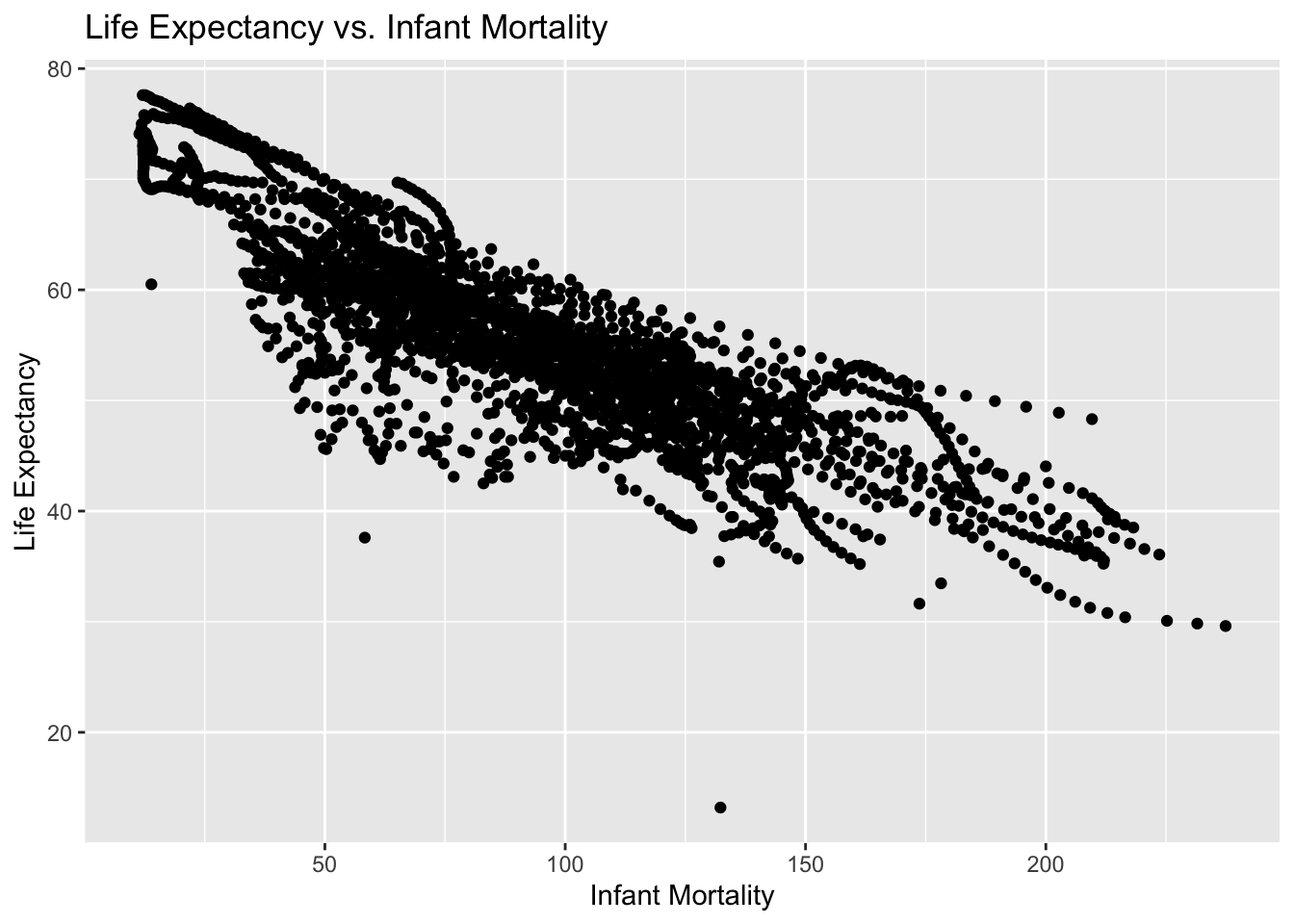
#Using the new variables you created, plot life expectancy as a function of infant mortality and as a function of population size. 
#Make two separate plots. 
#Plot the data as points. For the plot with population size on the x-axis, set the x-axis to a log scale.
# Plot life expectancy as a function of infant mortality

# using ggplot2 package to plot 
plot1 <- ggplot(subset1, aes(x = infant_mortality, y = life_expectancy)) +
  geom_point() +
  labs(title = "Life Expectancy vs. Infant Mortality",
       x = "Infant Mortality",
       y = "Life Expectancy")
plot1

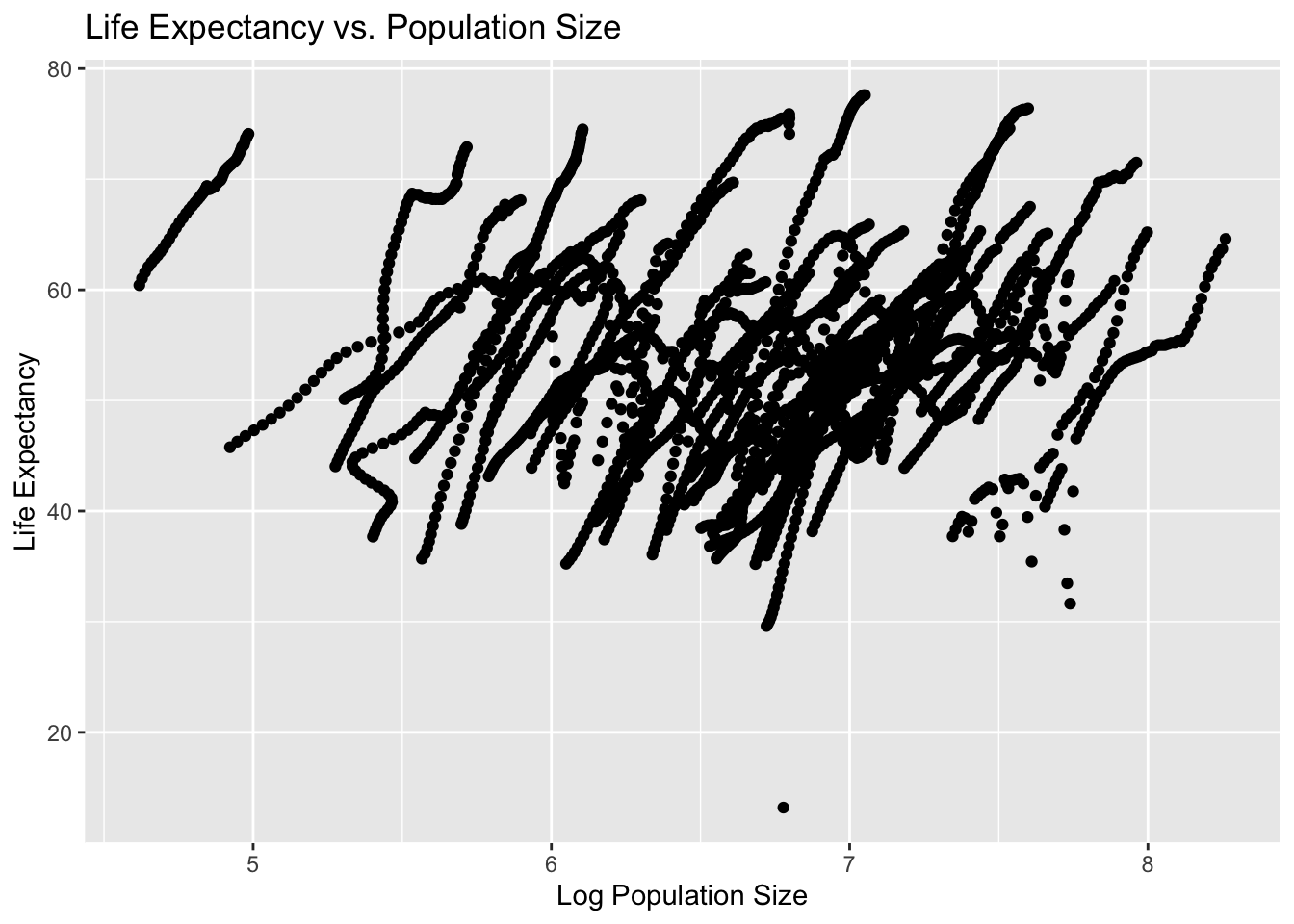
Warning: Removed 226 rows containing missing values (`geom_point()`).

# Plot life expectancy as a function of population size (log scale on x-axis)
plot2 <- ggplot(subset2, aes(x = log10(population), y = life_expectancy)) +
  geom_point() +
  labs(title = "Life Expectancy vs. Population Size",
       x = "Log Population Size",
       y = "Life Expectancy")
plot2

Warning: Removed 51 rows containing missing values (`geom_point()`).

More data processing

# Identify years with missing data for infant mortality
years_with_missing_data <- unique(africadata$year[is.na(africadata$infant_mortality)])
years_with_missing_data

 [1] 1960 1961 1962 1963 1964 1965 1966 1967 1968 1969 1970 1971 1972 1973 1974
[16] 1975 1976 1977 1978 1979 1980 1981 2016

# Choose the year 2000 and create a new object
africadata_2000 <- africadata[africadata$year == 2000, ]

# Display the structure of africadata_2000
str(africadata_2000)

'data.frame':   51 obs. of  9 variables:
 $ country         : Factor w/ 185 levels "Albania","Algeria",..: 2 3 18 22 26 27 29 31 32 33 ...
 $ year            : int  2000 2000 2000 2000 2000 2000 2000 2000 2000 2000 ...
 $ infant_mortality: num  33.9 128.3 89.3 52.4 96.2 ...
 $ life_expectancy : num  73.3 52.3 57.2 47.6 52.6 46.7 54.3 68.4 45.3 51.5 ...
 $ fertility       : num  2.51 6.84 5.98 3.41 6.59 7.06 5.62 3.7 5.45 7.35 ...
 $ population      : num  31183658 15058638 6949366 1736579 11607944 ...
 $ gdp             : num  5.48e+10 9.13e+09 2.25e+09 5.63e+09 2.61e+09 ...
 $ continent       : Factor w/ 5 levels "Africa","Americas",..: 1 1 1 1 1 1 1 1 1 1 ...
 $ region          : Factor w/ 22 levels "Australia and New Zealand",..: 11 10 20 17 20 5 10 20 10 10 ...

# Display summary statistics of africadata_2000
summary(africadata_2000)

         country        year      infant_mortality life_expectancy
 Algeria     : 1   Min.   :2000   Min.   : 12.30   Min.   :37.60  
 Angola      : 1   1st Qu.:2000   1st Qu.: 60.80   1st Qu.:51.75  
 Benin       : 1   Median :2000   Median : 80.30   Median :54.30  
 Botswana    : 1   Mean   :2000   Mean   : 78.93   Mean   :56.36  
 Burkina Faso: 1   3rd Qu.:2000   3rd Qu.:103.30   3rd Qu.:60.00  
 Burundi     : 1   Max.   :2000   Max.   :143.30   Max.   :75.00  
 (Other)     :45                                                  
   fertility       population             gdp               continent 
 Min.   :1.990   Min.   :    81154   Min.   :2.019e+08   Africa  :51  
 1st Qu.:4.150   1st Qu.:  2304687   1st Qu.:1.274e+09   Americas: 0  
 Median :5.550   Median :  8799165   Median :3.238e+09   Asia    : 0  
 Mean   :5.156   Mean   : 15659800   Mean   :1.155e+10   Europe  : 0  
 3rd Qu.:5.960   3rd Qu.: 17391242   3rd Qu.:8.654e+09   Oceania : 0  
 Max.   :7.730   Max.   :122876723   Max.   :1.329e+11                
                                                                      
                       region  
 Eastern Africa           :16  
 Western Africa           :16  
 Middle Africa            : 8  
 Northern Africa          : 6  
 Southern Africa          : 5  
 Australia and New Zealand: 0  
 (Other)                  : 0

More plotting

# Plot life expectancy as a function of infant mortality for the year 2000
plot_infant_mortality <- ggplot(africadata_2000, aes(x = infant_mortality, y = life_expectancy)) +
  geom_point() +
  geom_smooth(method = "lm", se = FALSE, color = "blue") +  # Add a fitted line
  labs(title = "Life Expectancy vs. Infant Mortality (Year 2000)",
       x = "Infant Mortality",
       y = "Life Expectancy") +
  theme_hc()
plot_infant_mortality

`geom_smooth()` using formula = 'y ~ x'

# Fit linear regression model for life expectancy vs. infant mortality
model_infant_mortality <- lm(life_expectancy ~ infant_mortality, data = africadata_2000)
summary(model_infant_mortality)


Call:
lm(formula = life_expectancy ~ infant_mortality, data = africadata_2000)

Residuals:
     Min       1Q   Median       3Q      Max 
-22.6651  -3.7087   0.9914   4.0408   8.6817 

Coefficients:
                 Estimate Std. Error t value Pr(>|t|)    
(Intercept)      71.29331    2.42611  29.386  < 2e-16 ***
infant_mortality -0.18916    0.02869  -6.594 2.83e-08 ***
---
Signif. codes:  0 '***' 0.001 '**' 0.01 '*' 0.05 '.' 0.1 ' ' 1

Residual standard error: 6.221 on 49 degrees of freedom
Multiple R-squared:  0.4701,    Adjusted R-squared:  0.4593 
F-statistic: 43.48 on 1 and 49 DF,  p-value: 2.826e-08

The linear regression model suggests a statistically significant negative relationship between infant mortality and life expectancy for the year 2000. As infant mortality increases, life expectancy is expected to decrease. The model explains a significant portion of the variability in life expectancy based on infant mortality.

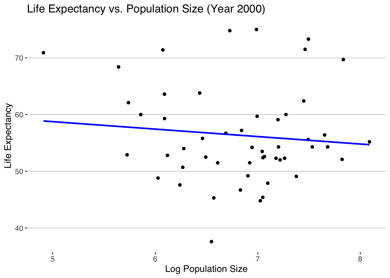
# Plot life expectancy as a function of population size (log scale on x-axis) for the year 2000
plot_population_size <- ggplot(africadata_2000, aes(x = log10(population), y = life_expectancy)) +
  geom_point() +
    geom_smooth(method = "lm", se = FALSE, color = "blue") +  # Add a fitted line
  labs(title = "Life Expectancy vs. Population Size (Year 2000)",
       x = "Log Population Size",
       y = "Life Expectancy") +
theme_hc()
plot_population_size

`geom_smooth()` using formula = 'y ~ x'

Simple model fits

# Fit linear regression model for life expectancy vs. log population size
model_population_size <- lm(life_expectancy ~ log10(population), data = africadata_2000)
summary(model_population_size)


Call:
lm(formula = life_expectancy ~ log10(population), data = africadata_2000)

Residuals:
    Min      1Q  Median      3Q     Max 
-19.113  -4.809  -1.554   3.907  18.863 

Coefficients:
                  Estimate Std. Error t value Pr(>|t|)    
(Intercept)         65.324     12.520   5.217 3.65e-06 ***
log10(population)   -1.315      1.829  -0.719    0.476    
---
Signif. codes:  0 '***' 0.001 '**' 0.01 '*' 0.05 '.' 0.1 ' ' 1

Residual standard error: 8.502 on 49 degrees of freedom
Multiple R-squared:  0.01044,   Adjusted R-squared:  -0.009755 
F-statistic: 0.517 on 1 and 49 DF,  p-value: 0.4755

The linear regression model suggests that, for the year 2000, there is not enough evidence to conclude a significant relationship between log-transformed population size and life expectancy. The coefficient for log-transformed population size is not statistically significant, and the model explains only a very small percentage of the variability in life expectancy.

# Fit linear regression model with life expectancy as the outcome and infant mortality as the predictor
fit_infant_mortality <- lm(life_expectancy ~ infant_mortality, data = africadata_2000)
summary(fit_infant_mortality)


Call:
lm(formula = life_expectancy ~ infant_mortality, data = africadata_2000)

Residuals:
     Min       1Q   Median       3Q      Max 
-22.6651  -3.7087   0.9914   4.0408   8.6817 

Coefficients:
                 Estimate Std. Error t value Pr(>|t|)    
(Intercept)      71.29331    2.42611  29.386  < 2e-16 ***
infant_mortality -0.18916    0.02869  -6.594 2.83e-08 ***
---
Signif. codes:  0 '***' 0.001 '**' 0.01 '*' 0.05 '.' 0.1 ' ' 1

Residual standard error: 6.221 on 49 degrees of freedom
Multiple R-squared:  0.4701,    Adjusted R-squared:  0.4593 
F-statistic: 43.48 on 1 and 49 DF,  p-value: 2.826e-08

The linear regression model for the year 2000 suggests a statistically significant negative relationship between infant mortality and life expectancy. As infant mortality increases, life expectancy is expected to decrease. The model explains a significant portion of the variability in life expectancy based on infant mortality.

# Fit linear regression model with life expectancy as the outcome and population size as the predictor
fit_population_size <- lm(life_expectancy ~ log10(population), data = africadata_2000)
summary(fit_population_size)


Call:
lm(formula = life_expectancy ~ log10(population), data = africadata_2000)

Residuals:
    Min      1Q  Median      3Q     Max 
-19.113  -4.809  -1.554   3.907  18.863 

Coefficients:
                  Estimate Std. Error t value Pr(>|t|)    
(Intercept)         65.324     12.520   5.217 3.65e-06 ***
log10(population)   -1.315      1.829  -0.719    0.476    
---
Signif. codes:  0 '***' 0.001 '**' 0.01 '*' 0.05 '.' 0.1 ' ' 1

Residual standard error: 8.502 on 49 degrees of freedom
Multiple R-squared:  0.01044,   Adjusted R-squared:  -0.009755 
F-statistic: 0.517 on 1 and 49 DF,  p-value: 0.4755

The linear regression model for the year 2000 suggests that there is not enough evidence to conclude a significant relationship between log-transformed population size and life expectancy. The coefficient for log-transformed population size is not statistically significant, and the model explains only a very small percentage of the variability in life expectancy.

This section is contributed by Chaohua Li

More data exploration (stars)

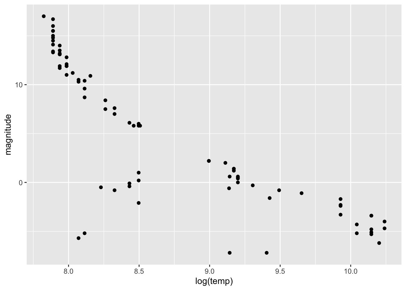
Choose dataset stars from the dslabs package. Details of variables in stars are listed below. 1. star: Name of star. 2. magnitude: Absolute magnitude of the star, which is a function of the star’s luminosity and distance to the star. 3. temp: Surface temperature in degrees Kelvin (K). 4. type: Spectral class of star in the OBAFGKM system.

#Load package dslabs and tidyverse
library("dslabs")
library("tidyverse")
#a preview of stars
head(stars)

            star magnitude temp type
1            Sun       4.8 5840    G
2        SiriusA       1.4 9620    A
3        Canopus      -3.1 7400    F
4       Arcturus      -0.4 4590    K
5 AlphaCentauriA       4.3 5840    G
6           Vega       0.5 9900    A

#check structure of stars
str(stars)

'data.frame':   96 obs. of  4 variables:
 $ star     : Factor w/ 95 levels "*40EridaniA",..: 87 85 48 38 33 92 49 79 77 47 ...
 $ magnitude: num  4.8 1.4 -3.1 -0.4 4.3 0.5 -0.6 -7.2 2.6 -5.7 ...
 $ temp     : int  5840 9620 7400 4590 5840 9900 5150 12140 6580 3200 ...
 $ type     : chr  "G" "A" "F" "K" ...

#check summary of stars
summary(stars)

          star      magnitude           temp           type          
 Altair     : 2   Min.   :-8.000   Min.   : 2500   Length:96         
 *40EridaniA: 1   1st Qu.:-1.800   1st Qu.: 3168   Class :character  
 *40EridaniB: 1   Median : 2.400   Median : 5050   Mode  :character  
 *40EridaniC: 1   Mean   : 4.257   Mean   : 8752                     
 *61CygniA  : 1   3rd Qu.:11.325   3rd Qu.: 9900                     
 *61CygniB  : 1   Max.   :17.000   Max.   :33600                     
 (Other)    :89

Processing data (stars)

Create star_ABKM which contains stars in the spectral classes of A/B/K/M 
(these classes have more than 10 stars).

#check frequencies for the spectral class of stars
table(stars$type)


 A  B DA DB DF  F  G  K  M  O 
13 19  2  1  1  7  4 16 32  1

#Create dataset star_ABKM that contains stars from spectral classes of A/B/K/M, as only these classes have more than 10 stars, and change type into a factor variable
star_ABKM  <- 
  stars %>% 
    filter(type %in% c("A","B","K","M")) %>%
      mutate(type=factor(type) )
#Check structure and summary of star_ABKM
str(star_ABKM)

'data.frame':   80 obs. of  4 variables:
 $ star     : Factor w/ 95 levels "*40EridaniA",..: 85 38 92 79 47 22 62 36 26 86 ...
 $ magnitude: num  1.4 -0.4 0.5 -7.2 -5.7 -2.4 -5.3 2.2 -0.8 -3.4 ...
 $ temp     : int  9620 4590 9900 12140 3200 20500 25500 8060 4130 25500 ...
 $ type     : Factor w/ 4 levels "A","B","K","M": 1 3 1 2 4 2 2 1 3 2 ...

summary(star_ABKM)

           star      magnitude           temp       type  
 Altair      : 2   Min.   :-7.200   Min.   : 2500   A:13  
 *40EridaniA : 1   1st Qu.:-1.225   1st Qu.: 2940   B:19  
 *40EridaniC : 1   Median : 2.200   Median : 4590   K:16  
 *61CygniA   : 1   Mean   : 4.645   Mean   : 8616   M:32  
 *61CygniB   : 1   3rd Qu.:11.900   3rd Qu.: 9900         
 *70OphiuchiA: 1   Max.   :17.000   Max.   :28000         
 (Other)     :73

Plotting (stars)

Plot absolute magnitude of a star as a function of log(surface temperature) and as a function of spectral class.

#Scatterplot: magnitude ~ log(temp)  
ggplot(star_ABKM, aes(log(temp), magnitude)) + 
  geom_point()

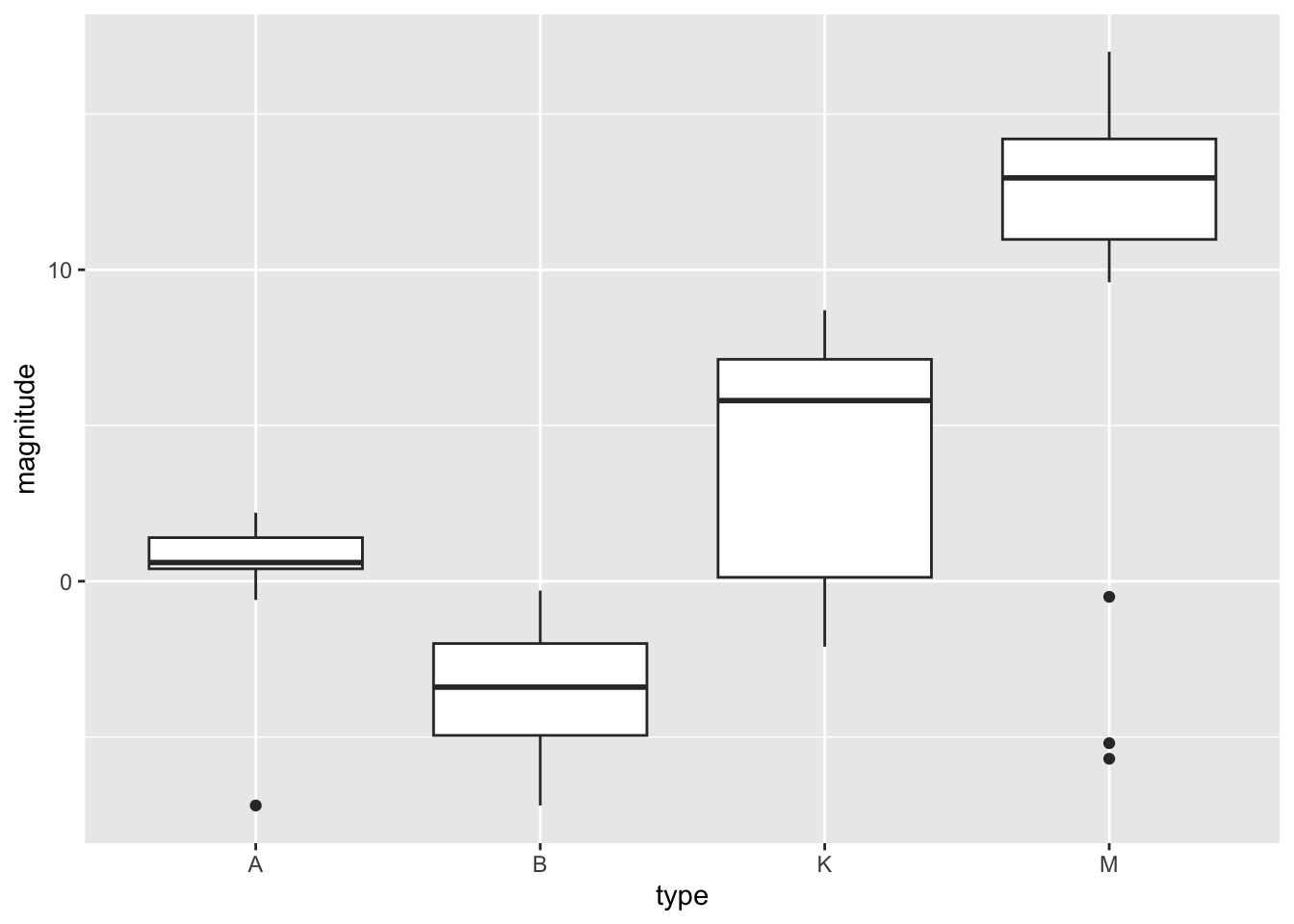
#Boxplot: magnitude ~ type  
ggplot(star_ABKM, aes(type, magnitude)) + 
  geom_boxplot()

Fit 2 simple linear models(stars)

Fit simple linear models with lm() function in R. Model 1: absolute magnitude 
as the outcome, and log(surface temperature) as the predictor; Model 2: 
absolute magnitude as the outcome, and spectral class as the predictor. 
Findings: Among stars of A/B/K/M spectral classes, 1 additional unit in the 
log(surface temperature) was significantly associated with a decrease of 7.6 
in the absolute magnitude (P-value<0.001); class K stars(P-value=0.014) and 
class M stars (P-value<0.001) had significantly higher absolute magnitude 
than class A stars; class B stars (P-value=0.009) had significantly lower 
absolute magnitude than class A stars.

#Linear model: magnitude~log(temp)
fit1<-lm(magnitude~log(temp), data=star_ABKM)
summary(fit1)


Call:
lm(formula = magnitude ~ log(temp), data = star_ABKM)

Residuals:
     Min       1Q   Median       3Q      Max 
-15.2219  -0.5008   0.8053   2.4234   5.7984 

Coefficients:
            Estimate Std. Error t value Pr(>|t|)    
(Intercept)  71.0185     4.9384   14.38   <2e-16 ***
log(temp)    -7.6195     0.5645  -13.50   <2e-16 ***
---
Signif. codes:  0 '***' 0.001 '**' 0.01 '*' 0.05 '.' 0.1 ' ' 1

Residual standard error: 4.048 on 78 degrees of freedom
Multiple R-squared:  0.7002,    Adjusted R-squared:  0.6964 
F-statistic: 182.2 on 1 and 78 DF,  p-value: < 2.2e-16

#Linear model: magnitude~type
fit2<-lm(magnitude~type, data=star_ABKM)
summary(fit2)


Call:
lm(formula = magnitude ~ type, data = star_ABKM)

Residuals:
    Min      1Q  Median      3Q     Max 
-17.184  -1.009   0.727   1.935   5.516 

Coefficients:
            Estimate Std. Error t value Pr(>|t|)    
(Intercept)   0.3615     1.1263   0.321  0.74909    
typeB        -3.8931     1.4616  -2.664  0.00944 ** 
typeK         3.7947     1.5163   2.503  0.01447 *  
typeM        11.1228     1.3356   8.328 2.59e-12 ***
---
Signif. codes:  0 '***' 0.001 '**' 0.01 '*' 0.05 '.' 0.1 ' ' 1

Residual standard error: 4.061 on 76 degrees of freedom
Multiple R-squared:  0.706, Adjusted R-squared:  0.6944 
F-statistic: 60.83 on 3 and 76 DF,  p-value: < 2.2e-16