Presentation Exercise

About Data

The data was about the poll that was conducted from Sept. 15 to Sept. 25 among a sample of U.S. citizens that oversampled young, Black and Hispanic respondents, with 8,327 respondents, and was weighted according to general population benchmarks for U.S. citizens from the U.S.

This the original Image to be reproduced

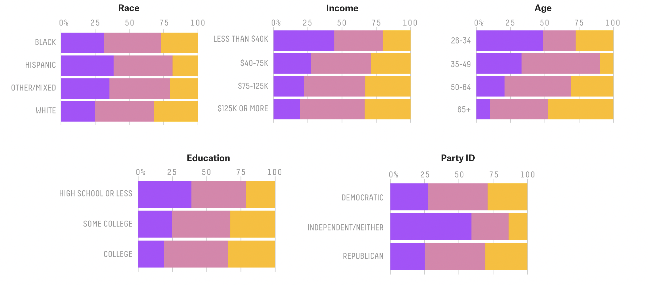
Prompted chatgpt for the code: Prompt: Please generate R code to visualize demographic data, including variables such as race, income, age, and education, segmented by voter category. Ensure that each variable is plotted as a bar graph with custom colors for the voter categories and arrange the plots in a grid with two columns. After I adjusted the code to try fit what I wanted.

# Suppress warnings while loading libraries
suppressPackageStartupMessages({
  library(flextable)
  library(ggplot2)
  library(gridExtra)
  library(readr)
  library(dplyr)
  library(patchwork)
})

# Read the CSV file without displaying column types
suppressMessages({
  nonvoters <- read_csv("nonvoters_data.csv", show_col_types = FALSE)
})

# Create a new categorical variable 'Age_Category' based on age ranges using mutate and ifelse
nonvoters <- nonvoters %>%
  mutate(Age = ifelse(ppage >= 26 & ppage <= 34, "26-34",
                               ifelse(ppage >= 35 & ppage <= 49, "35-49",
                                      ifelse(ppage >= 50 & ppage <= 64, "50-64", "65+"))))

# creating new labels for the party ID represented by Q30
nonvoters <- nonvoters %>%
  mutate(Q30 = case_when(
    Q30 == 1 ~ "DEMOCRATIC",
    Q30 == 2 ~ "REPUBLICAN",
    Q30 == 3 ~ "INDEPENDENT",
    TRUE ~ as.character(Q30)
  ))

# Define custom colors for voter categories
custom_colors <- c("#ffbc00", "#e082ad", "#ae4dff")

# Plot race by voter category
plot_race <- ggplot(nonvoters, aes(x = race, fill = voter_category)) +
  geom_bar(position = "fill") +
  labs(x = "Race", y = "Percentage", fill = "Voter Category") +
  scale_fill_manual(values = custom_colors) +
  theme_minimal() +
  theme(legend.position = "", axis.title.y = element_blank(), axis.title.x = element_blank()) +
  coord_flip() +
  ggtitle("Race") +
  theme(plot.title = element_text(hjust = 0.5))

# Plot income by voter category
plot_income <- ggplot(nonvoters, aes(x = income_cat, fill = voter_category)) +
  geom_bar(position = "fill") +
  labs(x = "Income", y = "Percentage", fill = "Voter Category") +
  scale_fill_manual(values = custom_colors) +
  theme_minimal() +
  theme(legend.position = "", axis.title.y = element_blank(), axis.title.x = element_blank()) +
  coord_flip() +
  ggtitle("Income") +
  theme(plot.title = element_text(hjust = 0.5))

# Plot Age by voter category
plot_age <- ggplot(nonvoters, aes(x = Age, fill = voter_category)) +
  geom_bar(position = "fill") +
  labs(x = "Age", y = "Percentage", fill = "Voter Category") +
  scale_fill_manual(values = custom_colors) +
  theme_minimal() +
  theme(legend.position = "", axis.title.y = element_blank(), axis.title.x = element_blank()) +
  coord_flip() +
  ggtitle("Age") +
  theme(plot.title = element_text(hjust = 0.5))

# Plot education by voter category
plot_education <- ggplot(nonvoters, aes(x = educ, fill = voter_category)) +
  geom_bar(position = "fill") +
  labs(x = "Education", y = "Percentage", fill = "Voter Category") +
  scale_fill_manual(values = custom_colors) +
  theme_minimal() +
  theme(legend.position = "", axis.title.y = element_blank(), axis.title.x = element_blank()) +
  coord_flip() +
  ggtitle("Education") +
  theme(plot.title = element_text(hjust = 0.5))

# Plot party id by voter category
plot_party <- ggplot(nonvoters, aes(x = Q30, fill = voter_category)) +
  geom_bar(position = "fill") +
  labs(x = "Party ID", y = "Percentage", fill = "") +
  scale_fill_manual(values = custom_colors) +
  theme_minimal() +
 theme(legend.position = "bottom", axis.title.y = element_blank(), axis.title.x = element_blank()) +
  coord_flip() +
  ggtitle("Party ID") +
  theme(plot.title = element_text(hjust = 0.5))

# Arrange plots in a grid
ggpubr::ggarrange   (plot_race + theme(aspect.ratio = 1),
          plot_income + theme(aspect.ratio = 1),
          plot_age + theme(aspect.ratio = 1),
          plot_education + theme(aspect.ratio = 1),
          plot_party + theme(aspect.ratio = 1))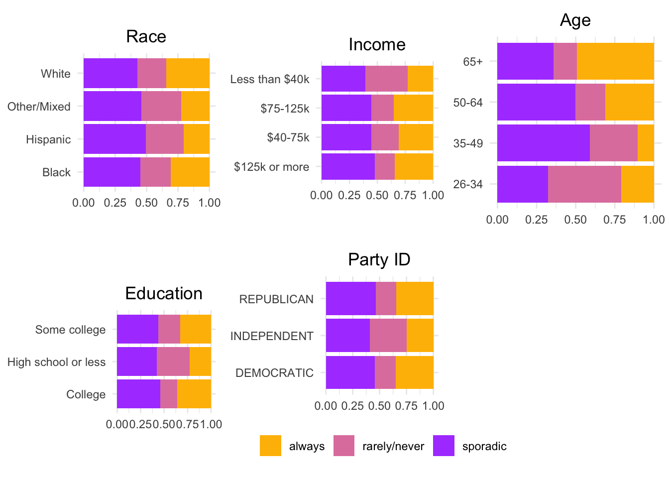

Nonvoters were more likely to have lower incomes; to be young; to have lower levels of education.

# Read WNBA player stats data from CSV file
suppressWarnings(wnba_player_stats <- read_csv("wnba-player-stats.csv", show_col_types = FALSE))

About Data

The data used contains season-level advanced stats for WNBA players by team for the 1997-2019 seasons, from Basketball-Reference.com. It also contains Composite Rating, which blends PER and Win Shares per 40 into a single metric that mimics RAPTOR player ratings. I prompted chatgpt that produced a code, I didn’t use it but it guided to write mine.

The original table to be reproduced.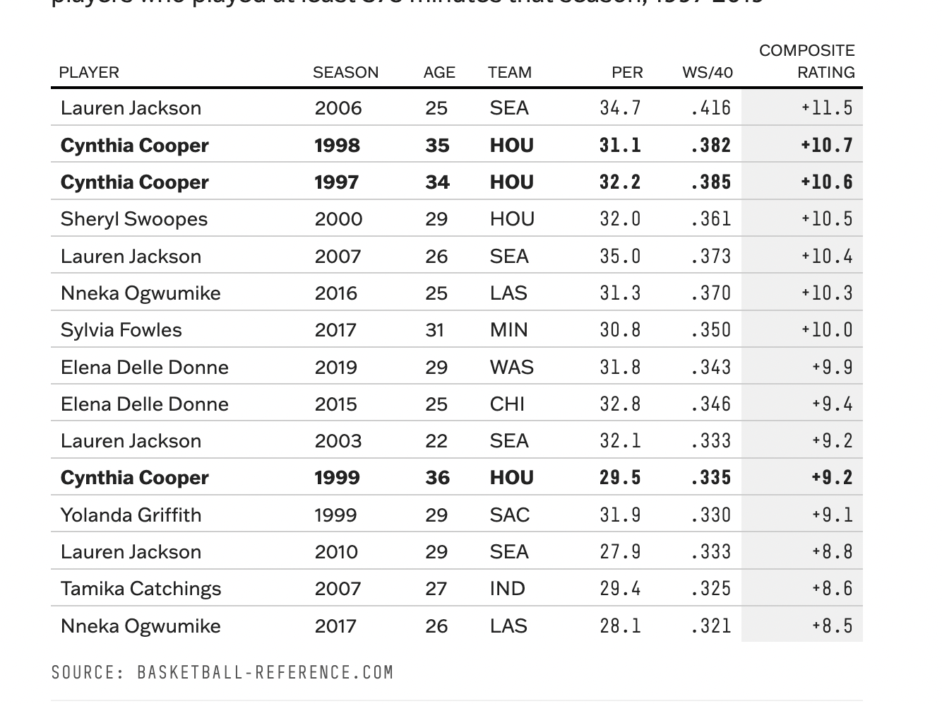

# Filter the data to include only players who played at least 375 minutes
filtered_data <- wnba_player_stats %>%
  filter(MP >= 375)

# Renaming variables to fit the table 
filtered_data <- filtered_data %>%
  rename(
    PLAYER = Player,
    SEASON = year_ID,
    AGE = Age,
    TEAM = Tm,
    WS40 = WS40,
    COMPOSITE_RATING = Composite_Rating
  )
# Arrange the data to find the best single-season composite ratings
top_players <- filtered_data %>%
  arrange(desc(COMPOSITE_RATING)) %>%
  select(PLAYER, SEASON, AGE, TEAM, PER, WS40, COMPOSITE_RATING) %>%
  head(15)

# Create flextable for the top players
ft <- flextable(top_players)

# Print the flextable
ft

PLAYER	SEASON	AGE	TEAM	PER	WS40	COMPOSITE_RATING
Lauren Jackson	2,006	25	SEA	34.7	0.416	11.5
Cynthia Cooper	1,998	35	HOU	31.1	0.382	10.7
Cynthia Cooper	1,997	34	HOU	32.2	0.385	10.6
Sheryl Swoopes	2,000	29	HOU	32.0	0.361	10.5
Lauren Jackson	2,007	26	SEA	35.0	0.373	10.4
Nneka Ogwumike	2,016	25	LAS	31.3	0.370	10.3
Sylvia Fowles	2,017	31	MIN	30.8	0.350	10.0
Elena Delle Donne	2,019	29	WAS	31.8	0.343	9.9
Elena Delle Donne	2,015	25	CHI	32.8	0.346	9.4
Lauren Jackson	2,003	22	SEA	32.1	0.333	9.2
Cynthia Cooper	1,999	36	HOU	29.5	0.335	9.2
Yolanda Griffith	1,999	29	SAC	31.9	0.330	9.1
Lauren Jackson	2,010	29	SEA	27.9	0.333	8.8
Tamika Catchings	2,007	27	IND	29.4	0.325	8.6
Nneka Ogwumike	2,017	26	LAS	28.1	0.321	8.5

The table shows Cooper-Dyke’s early WNBA seasons are among the best ever Best single-season composite ratings — based on a mix of player efficiency rating (PER) and win shares per 40 minutes — for WNBA players who played at least 375 minutes that season, 1997-2019